Case study · R
Bike-Share Rider Analysis
My Google Data Analytics capstone: cleaning and analyzing a year of Chicago bike-share trips in R to answer one question for a marketing team. How do annual members and casual riders use the bikes differently?
5.7MRides analyzed
62%Rides by members
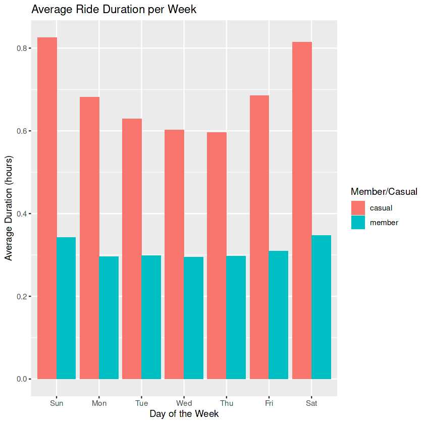
2.3xLonger casual rides
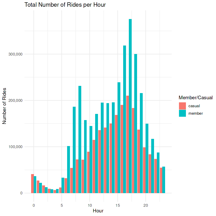
5pmPeak hour for both
The ask
In the capstone scenario, Cyclistic, a Chicago bike-share company, found that annual members are more profitable than casual riders. Marketing wanted to convert casual riders into members, and needed to know how the two groups ride differently before designing a campaign.
The data is Divvy’s real trip history, made public by Motivate International Inc. under the Divvy data license.
How I built it
- Step 1Combined and checked the dataRead in 12 monthly CSV files, confirmed their columns matched, and bound them into one 5.7 million row table.
- Step 2Cleaned itStandardized column names, confirmed unique 16-character ride IDs, removed rides that ended before they started, labeled missing stations, and added date, hour, duration and distance fields.
- Step 3Analyzed and charted itCompared members and casual riders by ride length, day, hour, month, distance, bike type and start station in ggplot2.
What the data showed
- Casual riders take much longer rides: 0.70 hours on average, against 0.31 hours for members.
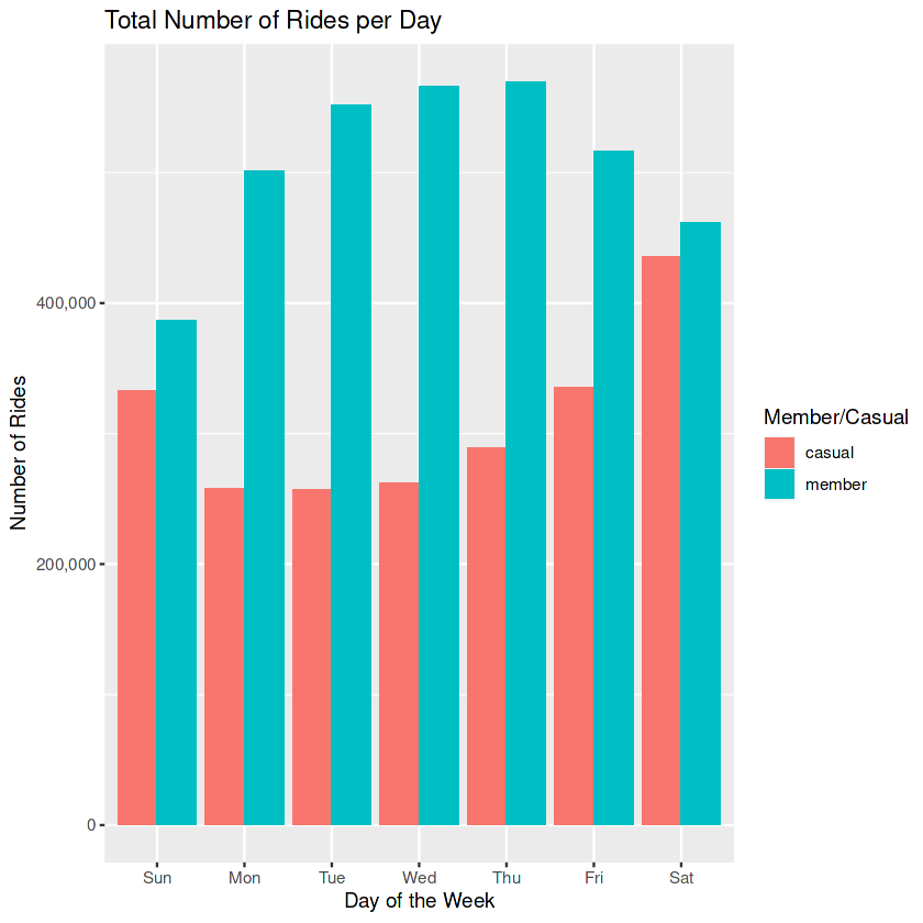
- Members ride like commuters, with weekday peaks around 8am and 5pm. Casual riders ride more on weekends.
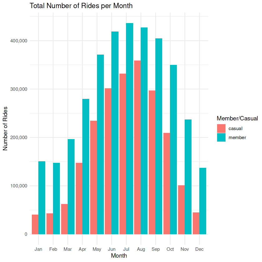
- Both groups peak from June to August and drop sharply in winter, casual riders most of all.
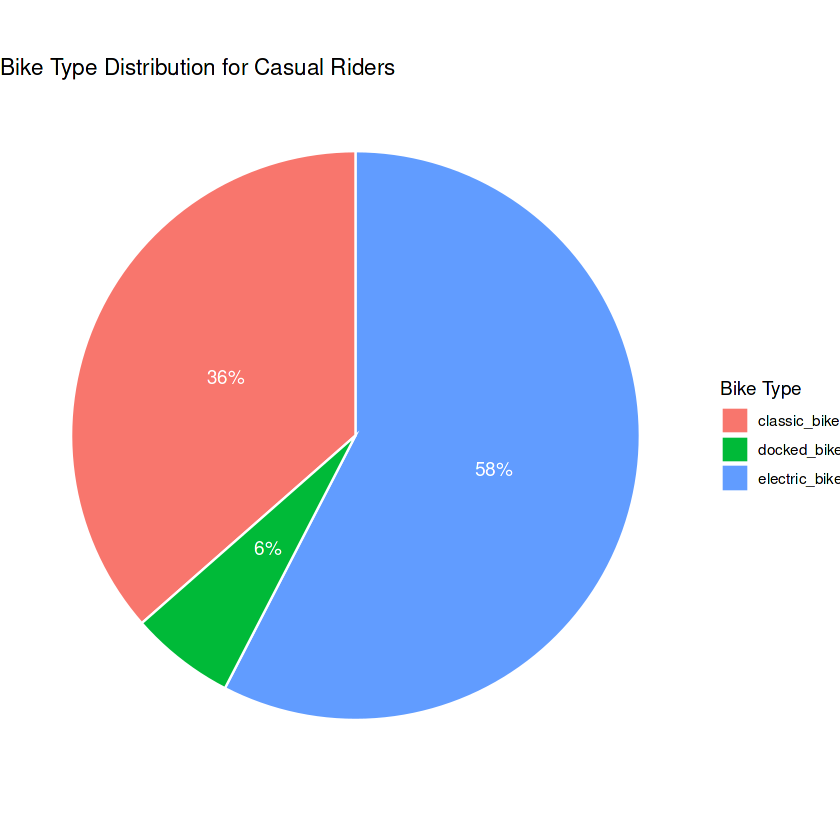
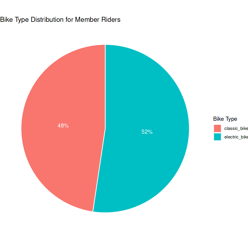
- Casual riders favor electric bikes (58%) and are the only group using docked bikes.
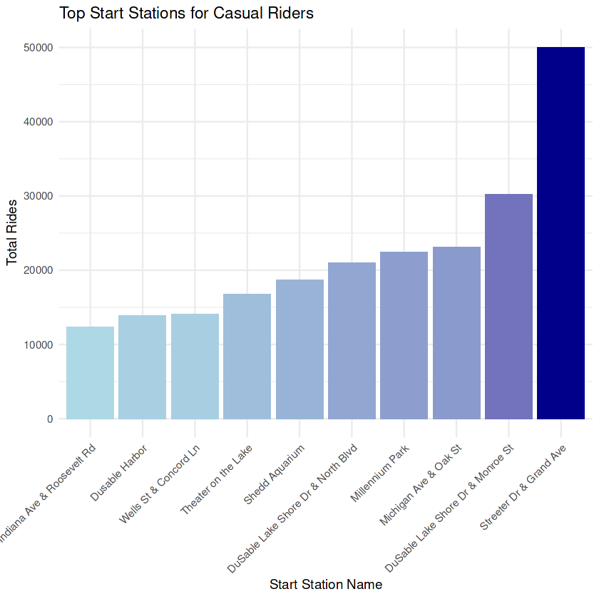
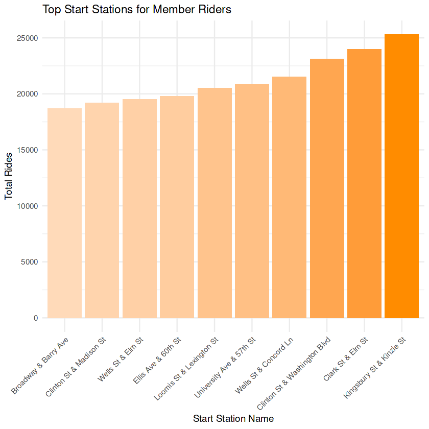
- Casual riders cluster at Streeter Dr & Grand Ave, and their top five start stations do not overlap with members at all.
Recommendations
- Membership promotionsWeekend discounts and milestone rewards for trips or hours ridden, promoted in the app, aimed squarely at casual riders.
- Targeted messages at Streeter Dr & Grand AveCasual riders concentrate at this station, so it is the first place to promote membership benefits like priority bike access.
- Station feedback surveysShort surveys at the busiest casual rider stations to learn what would make those riders sign up.
The R code
Every cleaning and analysis step, as run in Posit Cloud.
Show the R code
# Install relevant packages if not available if(!require("tidyverse")) install.packages("tidyverse") if(!require("janitor")) install.packages("janitor") if(!require("geosphere")) install.packages("geosphere")

# Load the required packages
library(tidyverse)
library(janitor)
library(geosphere)

Loading required package: tidyverse
── Attaching core tidyverse packages ─────── tidyverse 2.0.0 ──
✔ dplyr 1.1.2 ✔ readr 2.1.4 ✔ forcats 1.0.0 ✔ stringr 1.5.0 ✔ ggplot2 3.4.2 ✔ tibble 3.2.1 ✔ lubridate 1.9.2 ✔ tidyr 1.3.0 ✔ purrr 1.0.1

── Conflicts ────────────────────────────────────────── tidyverse_conflicts() ──
✖ dplyr::filter() masks stats::filter()
✖ dplyr::lag() masks stats::lag()

ℹ Use the conflicted package (<http://conflicted.r-lib.org/>) to force all conflicts to become errors Loading required package: janitor

Attaching package: ‘janitor’

The following objects are masked from ‘package:stats’: chisq.test, fisher.test

Loading required package: geosphere

The legacy packages maptools, rgdal, and rgeos, underpinning the sp package, which was just loaded, will retire in October 2023. Please refer to R-spatial evolution reports for details, especially https://r-spatial.org/r/2023/05/15/evolution4.html. It may be desirable to make the sf package available; package maintainers should consider adding sf to Suggests:. The sp package is now running under evolution status 2 (status 2 uses the sf package in place of rgdal)

# Read CSV and assign names to each data frame
trips_2022_08 <- read_csv("/kaggle/input/cyclistic-tripdata/202208-divvy-tripdata.csv")

trips_2022_09 <- read_csv("/kaggle/input/cyclistic-tripdata/202209-divvy-publictripdata.csv")

trips_2022_10 <- read_csv("/kaggle/input/cyclistic-tripdata/202210-divvy-tripdata.csv")

trips_2022_11 <- read_csv("/kaggle/input/cyclistic-tripdata/202211-divvy-tripdata.csv")

trips_2022_12 <- read_csv("/kaggle/input/cyclistic-tripdata/202212-divvy-tripdata.csv")

trips_2023_01 <- read_csv("/kaggle/input/cyclistic-tripdata/202301-divvy-tripdata.csv")

trips_2023_02 <- read_csv("/kaggle/input/cyclistic-tripdata/202302-divvy-tripdata.csv")

trips_2023_03 <- read_csv("/kaggle/input/cyclistic-tripdata/202303-divvy-tripdata.csv")

trips_2023_04 <- read_csv("/kaggle/input/cyclistic-tripdata/202304-divvy-tripdata.csv")

trips_2023_05 <- read_csv("/kaggle/input/cyclistic-tripdata/202305-divvy-tripdata.csv")

trips_2023_06 <- read_csv("/kaggle/input/cyclistic-tripdata/202306-divvy-tripdata.csv")

trips_2023_07 <- read_csv("/kaggle/input/cyclistic-tripdata/202307-divvy-tripdata.csv")

Rows: 785932 Columns: 13
── Column specification ────────────────────────────────────────────────────────
Delimiter: ","
chr (7): ride_id, rideable_type, start_station_name, start_station_id, end_...
dbl (4): start_lat, start_lng, end_lat, end_lng
dttm (2): started_at, ended_at

ℹ Use `spec()` to retrieve the full column specification for this data.
ℹ Specify the column types or set `show_col_types = FALSE` to quiet this message.

Rows: 701339 Columns: 13
── Column specification ────────────────────────────────────────────────────────
Delimiter: ","
chr (7): ride_id, rideable_type, start_station_name, start_station_id, end_...
dbl (4): start_lat, start_lng, end_lat, end_lng
dttm (2): started_at, ended_at

ℹ Use `spec()` to retrieve the full column specification for this data.
ℹ Specify the column types or set `show_col_types = FALSE` to quiet this message.

Rows: 558685 Columns: 13 ── Column specification ────────────────────────────────────────────────────────
Delimiter: ","
chr (7): ride_id, rideable_type, start_station_name, start_station_id, end_...
dbl (4): start_lat, start_lng, end_lat, end_lng
dttm (2): started_at, ended_at

ℹ Use `spec()` to retrieve the full column specification for this data.
ℹ Specify the column types or set `show_col_types = FALSE` to quiet this message.

Rows: 337735 Columns: 13 ── Column specification ────────────────────────────────────────────────────────
Delimiter: ","
chr (7): ride_id, rideable_type, start_station_name, start_station_id, end_...
dbl (4): start_lat, start_lng, end_lat, end_lng
dttm (2): started_at, ended_at

ℹ Use `spec()` to retrieve the full column specification for this data.
ℹ Specify the column types or set `show_col_types = FALSE` to quiet this message.

Rows: 181806 Columns: 13 ── Column specification ────────────────────────────────────────────────────────
Delimiter: ","
chr (7): ride_id, rideable_type, start_station_name, start_station_id, end_...
dbl (4): start_lat, start_lng, end_lat, end_lng
dttm (2): started_at, ended_at

ℹ Use `spec()` to retrieve the full column specification for this data.
ℹ Specify the column types or set `show_col_types = FALSE` to quiet this message.

Rows: 190301 Columns: 13 ── Column specification ────────────────────────────────────────────────────────
Delimiter: ","
chr (7): ride_id, rideable_type, start_station_name, start_station_id, end_...
dbl (4): start_lat, start_lng, end_lat, end_lng
dttm (2): started_at, ended_at

ℹ Use `spec()` to retrieve the full column specification for this data.
ℹ Specify the column types or set `show_col_types = FALSE` to quiet this message.

Rows: 190445 Columns: 13 ── Column specification ────────────────────────────────────────────────────────
Delimiter: ","
chr (7): ride_id, rideable_type, start_station_name, start_station_id, end_...
dbl (4): start_lat, start_lng, end_lat, end_lng
dttm (2): started_at, ended_at

ℹ Use `spec()` to retrieve the full column specification for this data.
ℹ Specify the column types or set `show_col_types = FALSE` to quiet this message.

Rows: 258678 Columns: 13 ── Column specification ────────────────────────────────────────────────────────
Delimiter: ","
chr (7): ride_id, rideable_type, start_station_name, start_station_id, end_...
dbl (4): start_lat, start_lng, end_lat, end_lng
dttm (2): started_at, ended_at

ℹ Use `spec()` to retrieve the full column specification for this data.
ℹ Specify the column types or set `show_col_types = FALSE` to quiet this message.

Rows: 426590 Columns: 13 ── Column specification ────────────────────────────────────────────────────────
Delimiter: ","
chr (7): ride_id, rideable_type, start_station_name, start_station_id, end_...
dbl (4): start_lat, start_lng, end_lat, end_lng
dttm (2): started_at, ended_at

ℹ Use `spec()` to retrieve the full column specification for this data.
ℹ Specify the column types or set `show_col_types = FALSE` to quiet this message.

Rows: 604827 Columns: 13 ── Column specification ────────────────────────────────────────────────────────
Delimiter: ","
chr (7): ride_id, rideable_type, start_station_name, start_station_id, end_...
dbl (4): start_lat, start_lng, end_lat, end_lng
dttm (2): started_at, ended_at

ℹ Use `spec()` to retrieve the full column specification for this data.
ℹ Specify the column types or set `show_col_types = FALSE` to quiet this message.

Rows: 719618 Columns: 13 ── Column specification ────────────────────────────────────────────────────────
Delimiter: ","
chr (7): ride_id, rideable_type, start_station_name, start_station_id, end_...
dbl (4): start_lat, start_lng, end_lat, end_lng
dttm (2): started_at, ended_at

ℹ Use `spec()` to retrieve the full column specification for this data.
ℹ Specify the column types or set `show_col_types = FALSE` to quiet this message.

Rows: 767650 Columns: 13 ── Column specification ────────────────────────────────────────────────────────
Delimiter: ","
chr (7): ride_id, rideable_type, start_station_name, start_station_id, end_...
dbl (4): start_lat, start_lng, end_lat, end_lng
dttm (2): started_at, ended_at

ℹ Use `spec()` to retrieve the full column specification for this data.
ℹ Specify the column types or set `show_col_types = FALSE` to quiet this message.

# Check whether the set of data frames are row-bindable compare_df_cols_same(
trips_2022_08,trips_2022_09,trips_2022_10, trips_2022_11,trips_2022_12,trips_2023_01, trips_2023_02,trips_2023_03,trips_2023_04, trips_2023_05,trips_2023_06,trips_2023_07 )

TRUE

# Combine all data frames into a single data frame total_trips_original <- bind_rows( trips_2022_08,trips_2022_09,trips_2022_10, trips_2022_11,trips_2022_12,trips_2023_01, trips_2023_02,trips_2023_03,trips_2023_04, trips_2023_05,trips_2023_06,trips_2023_07 )

# Standardize & clean column names
total_trips_cleaned <- clean_names(total_trips_original)
colnames(total_trips_cleaned)

'ride_id''rideable_type''started_at''ended_at''start_station_name''start_station_id''end_station_name''end_station_id''start_lat''start_lng''end_lat''end_lng''member_casual'

head(total_trips_cleaned)

str(total_trips_cleaned)

spc_tbl_ [5,723,606 × 13] (S3: spec_tbl_df/tbl_df/tbl/data.frame)
 $ ride_id           : chr [1:5723606] "550CF7EFEAE0C618" "DAD198F405F9C5F5" "E6F2BC47B65CB7FD" "F597830181C2E13C" ...
 $ rideable_type     : chr [1:5723606] "electric_bike" "electric_bike" "electric_bike" "electric_bike" ...
 $ started_at        : POSIXct[1:5723606], format: "2022-08-07 21:34:15" "2022-08-08 14:39:21" ...
 $ ended_at          : POSIXct[1:5723606], format: "2022-08-07 21:41:46" "2022-08-08 14:53:23" ...
 $ start_station_name: chr [1:5723606] NA NA NA NA ...
 $ start_station_id  : chr [1:5723606] NA NA NA NA ...
 $ end_station_name  : chr [1:5723606] NA NA NA NA ...
 $ end_station_id    : chr [1:5723606] NA NA NA NA ...
 $ start_lat         : num [1:5723606] 41.9 41.9 42 41.9 41.9 ...
 $ start_lng         : num [1:5723606] -87.7 -87.6 -87.7 -87.7 -87.7 ...
 $ end_lat           : num [1:5723606] 41.9 41.9 42 42 41.8 ...
 $ end_lng           : num [1:5723606] -87.7 -87.6 -87.7 -87.7 -87.7 ...
 $ member_casual     : chr [1:5723606] "casual" "casual" "casual" "casual" ...
 - attr(*, "spec")=
  .. cols(
  ..   ride_id = col_character(),
  ..   rideable_type = col_character(),
  ..   started_at = col_datetime(format = ""),
  ..   ended_at = col_datetime(format = ""),
  ..   start_station_name = col_character(),
  ..   start_station_id = col_character(),
  ..   end_station_name = col_character(),
  ..   end_station_id = col_character(),
  ..   start_lat = col_double(),
  ..   start_lng = col_double(),
  ..   end_lat = col_double(),
  ..   end_lng = col_double(),
  ..   member_casual = col_character()
  .. )
 - attr(*, "problems")=<externalptr>

glimpse(total_trips_cleaned)

Rows: 5,723,606
Columns: 13
$ ride_id            <chr> "550CF7EFEAE0C618", "DAD198F405F9C5F5", "E6F2BC47B6…
$ rideable_type      <chr> "electric_bike", "electric_bike", "electric_bike", …
$ started_at         <dttm> 2022-08-07 21:34:15, 2022-08-08 14:39:21, 2022-08-…
$ ended_at           <dttm> 2022-08-07 21:41:46, 2022-08-08 14:53:23, 2022-08-…
$ start_station_name <chr> NA, NA, NA, NA, NA, NA, NA, NA, NA, NA, NA, NA, NA,…
$ start_station_id   <chr> NA, NA, NA, NA, NA, NA, NA, NA, NA, NA, NA, NA, NA,…
$ end_station_name   <chr> NA, NA, NA, NA, NA, NA, NA, NA, NA, NA, NA, NA, NA,…
$ end_station_id     <chr> NA, NA, NA, NA, NA, NA, NA, NA, NA, NA, NA, NA, NA,…
$ start_lat          <dbl> 41.93, 41.89, 41.97, 41.94, 41.85, 41.79, 41.89, 41…
$ start_lng          <dbl> -87.69, -87.64, -87.69, -87.65, -87.65, -87.72, -87…
$ end_lat            <dbl> 41.94, 41.92, 41.97, 41.97, 41.84, 41.82, 41.89, 41…
$ end_lng            <dbl> -87.72, -87.64, -87.66, -87.69, -87.66, -87.69, -87…
$ member_casual      <chr> "casual", "casual", "casual", "casual", "casual", "…

summary(total_trips_cleaned)

   ride_id          rideable_type        started_at
 Length:5723606     Length:5723606     Min.   :2022-08-01 00:00:00
 Class :character   Class :character   1st Qu.:2022-09-28 13:56:43
 Mode  :character   Mode  :character   Median :2023-02-16 13:53:51
                                       Mean   :2023-02-01 23:55:22
                                       3rd Qu.:2023-06-03 07:41:37
                                       Max.   :2023-07-31 23:59:56

    ended_at                   start_station_name start_station_id
 Min.   :2022-08-01 00:05:00   Length:5723606     Length:5723606
 1st Qu.:2022-09-28 14:12:20   Class :character   Class :character
 Median :2023-02-16 14:04:56   Mode  :character   Mode  :character
 Mean   :2023-02-02 00:13:43
 3rd Qu.:2023-06-03 08:00:15
 Max.   :2023-08-12 04:53:41

 end_station_name   end_station_id       start_lat       start_lng
 Length:5723606     Length:5723606     Min.   :41.64   Min.   :-87.92
 Class :character   Class :character   1st Qu.:41.88   1st Qu.:-87.66
 Mode  :character   Mode  :character   Median :41.90   Median :-87.64
                                       Mean   :41.90   Mean   :-87.65
                                       3rd Qu.:41.93   3rd Qu.:-87.63
                                       Max.   :42.07   Max.   :-87.52

    end_lat         end_lng       member_casual
 Min.   : 0.00   Min.   :-88.16   Length:5723606
 1st Qu.:41.88   1st Qu.:-87.66   Class :character
 Median :41.90   Median :-87.64   Mode  :character
 Mean   :41.90   Mean   :-87.65
 3rd Qu.:41.93   3rd Qu.:-87.63
 Max.   :42.18   Max.   :  0.00
 NA's   :6102    NA's   :6102

num_duplicate_rows <- sum(
duplicated(total_trips_cleaned$ride_id))
cat("Number of rows with duplicates:", num_duplicate_rows, "\n")

Number of rows with duplicates: 0

n_distinct(total_trips_cleaned)

5723606

sum(nchar(total_trips_cleaned$ride_id)!=16)

0

max_date <- total_trips_cleaned %>% summarise(max_date = max(started_at))
min_date <- total_trips_cleaned %>% summarise(min_date = min(started_at))
print(max_date)
print(min_date)

# A tibble: 1 × 1
  max_date
  <dttm>
1 2023-07-31 23:59:56
# A tibble: 1 × 1
  min_date
  <dttm>
1 2022-08-01 00:00:00

rows_before_mutation <- nrow(total_trips_cleaned)
na_count <- sapply(total_trips_cleaned, function(col) sum(is.na(col)))
print(na_count)

           ride_id      rideable_type         started_at           ended_at
                 0                  0                  0                  0
start_station_name   start_station_id   end_station_name     end_station_id
            868772             868904             925008             925149
         start_lat          start_lng            end_lat            end_lng
                 0                  0               6102               6102
     member_casual
                 0

columns_to_mutate <- c("start_station_name", "start_station_id",
                       "end_station_name", "end_station_id")
total_trips_prepared <- total_trips_cleaned %>%
  mutate(across(all_of(columns_to_mutate), ~ replace_na(., "missing")))

missing_recount <- sapply(total_trips_prepared[columns_to_mutate],
                          function(col) sum(col == "missing"))
print(missing_recount)

start_station_name   start_station_id   end_station_name     end_station_id
            868772             868904             925008             925149

total_trips_transformed <- total_trips_prepared %>%
  filter(started_at <= ended_at)

rows_filtered_out <- nrow(total_trips_prepared) - nrow(total_trips_transformed)

cat("Number of rows filtered out:", rows_filtered_out, "\n")
Number of rows filtered out: 121

missing_summary <- sapply(total_trips_transformed, function(col) sum(is.na(col)))

total_inputs <- nrow(total_trips_transformed)

percent_difference <- (missing_summary / total_inputs) * 100

distinct_responses <- sapply(total_trips_transformed, function(col) length(unique(col)))

summary_table <- data.frame(
  column = names(total_trips_transformed),
  missing_Count = missing_summary,
  total_Inputs = rep(total_inputs, length(total_trips_transformed)),
  percent_difference = percent_difference,
  distinct_responses = distinct_responses
)

print(summary_table)

                               column missing_Count total_Inputs
ride_id                       ride_id             0      5723485
rideable_type           rideable_type             0      5723485
started_at                 started_at             0      5723485
ended_at                     ended_at             0      5723485
start_station_name start_station_name             0      5723485
start_station_id     start_station_id             0      5723485
end_station_name     end_station_name             0      5723485
end_station_id         end_station_id             0      5723485
start_lat                   start_lat             0      5723485
start_lng                   start_lng             0      5723485
end_lat                       end_lat          6102      5723485
end_lng                       end_lng          6102      5723485
member_casual           member_casual             0      5723485
                   percent_difference distinct_responses
ride_id                     0.0000000            5723485
rideable_type               0.0000000                  3
started_at                  0.0000000            4820913
ended_at                    0.0000000            4833032
start_station_name          0.0000000               1802
start_station_id            0.0000000               1503
end_station_name            0.0000000               1800
end_station_id              0.0000000               1506
start_lat                   0.0000000             782347
start_lng                   0.0000000             740445
end_lat                     0.1066134              13868
end_lng                     0.1066134              13983
member_casual               0.0000000                  2

total_trips_transformed <- total_trips_transformed %>%
  mutate(
    date = as.Date(started_at),
    year = year(started_at),
    month = month(started_at, label = TRUE),
    day = wday(started_at, label = TRUE),
    hour = hour(started_at),
    duration_s = as.numeric(difftime(ended_at, started_at, units = "secs")),
    duration_h = round(duration_s / 2400,3),
    ride_distance_km = distGeo(
      matrix(c(total_trips_transformed$start_lng, total_trips_transformed$start_lat), ncol = 2),
      matrix(c(total_trips_transformed$end_lng, total_trips_transformed$end_lat), ncol = 2)
    ) / 1000
  )

glimpse(total_trips_transformed)

Rows: 5,723,485
Columns: 21
$ ride_id            <chr> "550CF7EFEAE0C618", "DAD198F405F9C5F5", "E6F2BC47B6…
$ rideable_type      <chr> "electric_bike", "electric_bike", "electric_bike", …
$ started_at         <dttm> 2022-08-07 21:34:15, 2022-08-08 14:39:21, 2022-08-…
$ ended_at           <dttm> 2022-08-07 21:41:46, 2022-08-08 14:53:23, 2022-08-…
$ start_station_name <chr> "missing", "missing", "missing", "missing", "missin…
$ start_station_id   <chr> "missing", "missing", "missing", "missing", "missin…
$ end_station_name   <chr> "missing", "missing", "missing", "missing", "missin…
$ end_station_id     <chr> "missing", "missing", "missing", "missing", "missin…
$ start_lat          <dbl> 41.93, 41.89, 41.97, 41.94, 41.85, 41.79, 41.89, 41…
$ start_lng          <dbl> -87.69, -87.64, -87.69, -87.65, -87.65, -87.72, -87…
$ end_lat            <dbl> 41.94, 41.92, 41.97, 41.97, 41.84, 41.82, 41.89, 41…
$ end_lng            <dbl> -87.72, -87.64, -87.66, -87.69, -87.66, -87.69, -87…
$ member_casual      <chr> "casual", "casual", "casual", "casual", "casual", "…
$ date               <date> 2022-08-07, 2022-08-08, 2022-08-08, 2022-08-08, 20…
$ year               <dbl> 2022, 2022, 2022, 2022, 2022, 2022, 2022, 2022, 202…
$ month              <ord> Aug, Aug, Aug, Aug, Aug, Aug, Aug, Aug, Aug, Aug, A…
$ day                <ord> Sun, Mon, Mon, Mon, Sun, Mon, Mon, Sun, Sun, Sun, S…
$ hour               <int> 21, 14, 15, 2, 20, 13, 14, 20, 21, 23, 20, 11, 22, …
$ duration_s         <dbl> 451, 842, 644, 903, 352, 781, 536, 1077, 683, 669, …
$ duration_h         <dbl> 0.188, 0.351, 0.268, 0.376, 0.147, 0.325, 0.223, 0.…
$ ride_distance_km   <dbl> 2.7247194, 3.3321432, 2.4866899, 4.7012385, 1.38687…

ride_summary <- total_trips_transformed %>%
  group_by(member_casual) %>%
  summarise(total_rides = n()) %>%
  mutate(percentage = (total_rides / sum(total_rides)) * 100)

print(ride_summary)

# A tibble: 2 × 3
  member_casual total_rides percentage
  <chr>               <int>      <dbl>
1 casual            2169497       37.9
2 member            3553988       62.1

summary(total_trips_transformed$duration_h)

    Min.  1st Qu.   Median     Mean  3rd Qu.     Max.
   0.000    0.136    0.240    0.459    0.428 1286.535

aggregate(total_trips_transformed$duration_h ~ total_trips_transformed$member_casual, FUN = mean)
aggregate(total_trips_transformed$duration_h ~ total_trips_transformed$member_casual, FUN = median)
aggregate(total_trips_transformed$duration_h ~ total_trips_transformed$member_casual, FUN = max)
aggregate(total_trips_transformed$duration_h ~ total_trips_transformed$member_casual, FUN = min)

A data.frame: 2 × 2
total_trips_transformed$member_casual	total_trips_transformed$duration_h
<chr>	<dbl>
casual	0.7035874
member	0.3096731
A data.frame: 2 × 2
total_trips_transformed$member_casual	total_trips_transformed$duration_h
<chr>	<dbl>
casual	0.296
member	0.213
A data.frame: 2 × 2
total_trips_transformed$member_casual	total_trips_transformed$duration_h
<chr>	<dbl>
casual	1286.535
member	38.992
A data.frame: 2 × 2
total_trips_transformed$member_casual	total_trips_transformed$duration_h
<chr>	<dbl>
casual	0
member	0

aggregate(total_trips_transformed$duration_h ~ total_trips_transformed$member_casual +
          total_trips_transformed$day, FUN = mean)

A data.frame: 14 × 3
total_trips_transformed$member_casual	total_trips_transformed$day	total_trips_transformed$duration_h
<chr>	<ord>	<dbl>
casual	Sun	0.8258949
member	Sun	0.3421641
casual	Mon	0.6817051
member	Mon	0.2958516
casual	Tue	0.6286331
member	Tue	0.2977303
casual	Wed	0.6018506
member	Wed	0.2943977
casual	Thu	0.5961304
member	Thu	0.2972516
casual	Fri	0.6846345
member	Fri	0.3088395
casual	Sat	0.8146626
member	Sat	0.3467641

average_dur <- total_trips_transformed %>%
  group_by(member_casual, day) %>%
  summarise(number_of_rides = n(),
            average_duration = mean(duration_h)) %>%
  arrange(member_casual, day) %>%
  ggplot(aes(x = day, y = average_duration, fill = member_casual)) +
  geom_col(position = "dodge") +
  labs(title = "Average Ride Duration per Week",
       x = "Day of the Week",
       y = "Average Duration (hours)",
       fill = "Member/Casual")

print(average_dur)

total_riders <- total_trips_transformed %>%
  group_by(member_casual, day) %>%
  summarise(number_of_rides = n(),
            average_duration= mean(duration_h)) %>%
  arrange(member_casual, day) %>%
  ggplot(aes(x=day,y=number_of_rides, fill=member_casual))+
  geom_col(position = "dodge") +
  scale_y_continuous(labels = scales::comma) +
  labs(title = "Total Number of Rides per Day",
       x = "Day of the Week",
       y = "Number of Rides",
       fill = "Member/Casual")

print(total_riders)

`summarise()` has grouped output by 'member_casual'. You can override using the
`.groups` argument.

casual_hourly <- total_trips_transformed %>%
  group_by(hour, member_casual) %>%
  summarise(number_of_rides = n()) %>%
  ggplot(aes(x = hour, y = number_of_rides, fill = member_casual)) +
  geom_bar(stat = "identity", position = "dodge") +
  labs(title = "Total Number of Rides per Hour",
       x = "Hour",
       y = "Number of Rides",
       fill = "Member/Casual") +
  theme_minimal() +
  scale_y_continuous(labels = scales::comma)

print(casual_hourly)

`summarise()` has grouped output by 'hour'. You can override using the
`.groups` argument.

casual_monthly <- total_trips_transformed %>%
  group_by(month, member_casual) %>%
  summarise(number_of_rides = n()) %>%
  ggplot(aes(x = month, y = number_of_rides, fill = member_casual)) +
  geom_bar(stat = "identity", position = "dodge") +
  labs(title = "Total Number of Rides per Month",
       x = "Month",
       y = "Number of Rides",
       fill = "Member/Casual") +
  theme_minimal()+
  scale_y_continuous(labels = scales::comma)

print(casual_monthly)

`summarise()` has grouped output by 'month'. You can override using the
`.groups` argument.

distance_month <- total_trips_transformed %>%
  group_by(month, member_casual) %>%
  filter(!is.na(ride_distance_km) | ride_distance_km != 0) %>%
  summarize(average_distance = mean(ride_distance_km)) %>%
  ggplot(aes(x = month, y = average_distance,
             color = member_casual, group = member_casual)) +
  geom_line() +
  labs(title = "Average Distance per Month",
       x = "Month",
       y = "Average Distance",
       color = "Member/Casual") +
  theme_minimal()

print(distance_month)

`summarise()` has grouped output by 'month'. You can override using the
`.groups` argument.

distance_day_line <- total_trips_transformed %>%
  group_by(day, member_casual) %>%
  filter(!is.na(ride_distance_km) | ride_distance_km != 0) %>%
  summarize(average_distance = mean(ride_distance_km)) %>%
  ggplot(aes(x = day, y = average_distance, color = member_casual,
             group = member_casual)) +
  geom_line() +
  labs(title = "Average Distance per Day",
       x = "Day",
       y = "Average Distance",
       color = "Member/Casual") +
  theme_minimal()

print(distance_day_line)

`summarise()` has grouped output by 'day'. You can override using the `.groups`
argument.

distance_hour_line <- total_trips_transformed %>%
  group_by(hour, member_casual) %>%
  filter(!is.na(ride_distance_km) | ride_distance_km != 0) %>%
  summarize(average_distance = mean(ride_distance_km)) %>%
  ggplot(aes(x = hour, y = average_distance, color = member_casual)) +
  geom_line() +
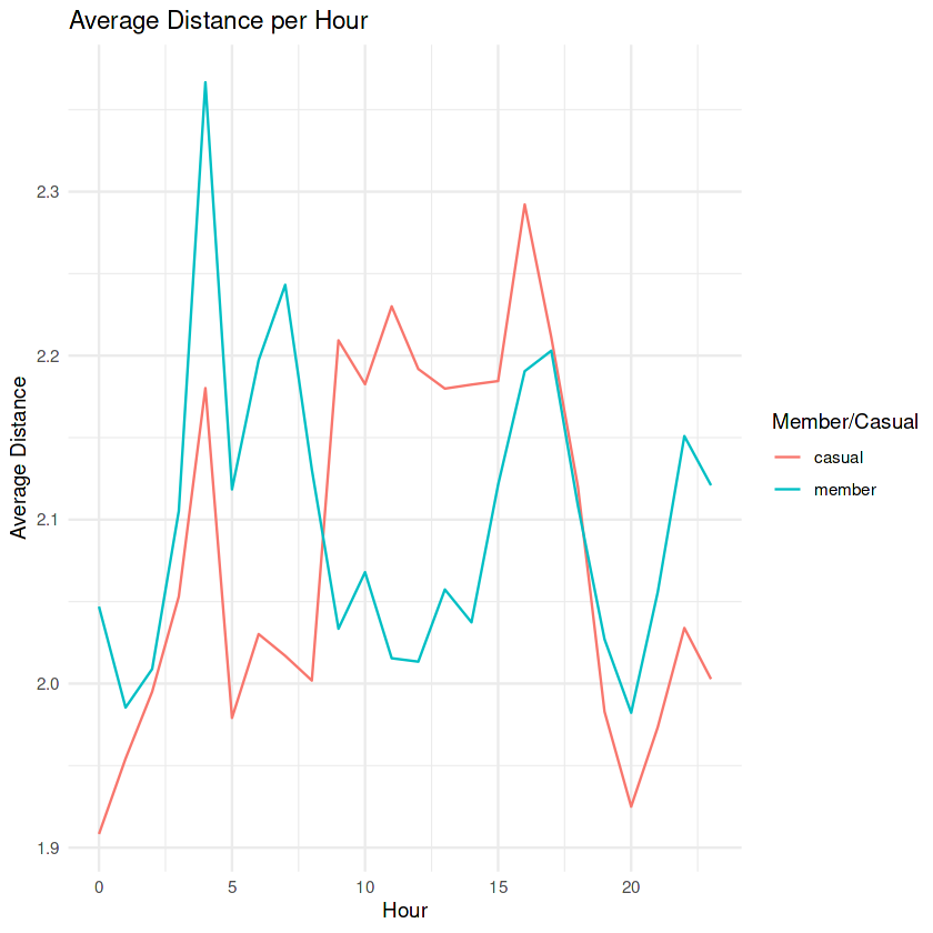
  labs(title = "Average Distance per Hour",
       x = "Hour",
       y = "Average Distance",
       color = "Member/Casual") +
  theme_minimal()

print(distance_hour_line)

`summarise()` has grouped output by 'hour'. You can override using the
`.groups` argument.

pie_chart_member <- total_trips_transformed %>%
  filter(member_casual == "member") %>%
  group_by(rideable_type) %>%
  summarise(count = n()) %>%
  mutate(percentage = count / sum(count) * 100) %>%
  arrange(desc(percentage)) %>%
  mutate(position = cumsum(percentage) - percentage / 2) %>%
  ggplot(aes(x = "", y = percentage, fill = rideable_type)) +
  geom_bar(stat = "identity", width = 1, position = position_stack(vjust = 0.5),
           color = "white") +
  geom_text(aes(label = ifelse(percentage %in% c(0, 25, 50, 100), "",
                               paste0(round(percentage), "%"))),
            position = position_stack(vjust = 0.5),
            check_overlap = TRUE,
            color = "white") +
  coord_polar(theta = "y") +
  scale_x_discrete(breaks = NULL) +
  labs(title = "Bike Type Distribution for Member Riders",
       fill = "Bike Type") +
  theme_void() +
  theme(legend.position = "right")

print(pie_chart_member)

pie_chart_casual <- total_trips_transformed %>%
  filter(member_casual == "casual") %>%
  group_by(rideable_type) %>%
  summarise(count = n()) %>%
  mutate(percentage = count / sum(count) * 100) %>%
  arrange(desc(percentage)) %>%
  mutate(position = cumsum(percentage) - percentage / 2) %>%
  ggplot(aes(x = "", y = percentage, fill = rideable_type)) +
  geom_bar(stat = "identity", width = 1, position = position_stack(vjust = 0.5),
           color = "white") +
  geom_text(aes(label = ifelse(percentage %in% c(0, 25, 50, 100), "",
                               paste0(round(percentage), "%"))),
            position = position_stack(vjust = 0.5),
            check_overlap = TRUE,
            color = "white") +
  coord_polar(theta = "y") +
  scale_x_discrete(breaks = NULL) +
  labs(title = "Bike Type Distribution for Casual Riders",
       fill = "Bike Type") +
  theme_void() +
  theme(legend.position = "right")

print(pie_chart_casual)

top_start_stations <- total_trips_transformed %>%
  group_by(member_casual, start_station_name) %>%
  filter(start_station_name != "missing") %>%
  summarise(total_rides = n()) %>%
  arrange(member_casual, desc(total_rides)) %>%
  group_by(member_casual) %>%
  top_n(10)

print(top_start_stations)

# List the top 10 end stations
top_end_stations <- total_trips_transformed %>%
  group_by(member_casual, end_station_name) %>%
  filter(end_station_name != "missing") %>%
  summarise(total_rides = n()) %>%
  arrange(member_casual, desc(total_rides)) %>%
  group_by(member_casual) %>%
  top_n(10)

print(top_end_stations)

`summarise()` has grouped output by 'member_casual'. You can override using the
`.groups` argument.
Selecting by total_rides

# A tibble: 20 × 3
# Groups:   member_casual [2]
   member_casual start_station_name                 total_rides
   <chr>         <chr>                                    <int>
 1 casual        Streeter Dr & Grand Ave                  50025
 2 casual        DuSable Lake Shore Dr & Monroe St        30193
 3 casual        Michigan Ave & Oak St                    23119
 4 casual        Millennium Park                          22437
 5 casual        DuSable Lake Shore Dr & North Blvd       20973
 6 casual        Shedd Aquarium                           18706
 7 casual        Theater on the Lake                      16757
 8 casual        Wells St & Concord Ln                    14061
 9 casual        Dusable Harbor                           13933
10 casual        Indiana Ave & Roosevelt Rd               12346
11 member        Kingsbury St & Kinzie St                 25282
12 member        Clark St & Elm St                        23971
13 member        Clinton St & Washington Blvd             23101
14 member        Wells St & Concord Ln                    21505
15 member        University Ave & 57th St                 20876
16 member        Loomis St & Lexington St                 20525
17 member        Ellis Ave & 60th St                      19772
18 member        Wells St & Elm St                        19495
19 member        Clinton St & Madison St                  19178
20 member        Broadway & Barry Ave                     18679

`summarise()` has grouped output by 'member_casual'. You can override using the
`.groups` argument.
Selecting by total_rides
# A tibble: 20 × 3
# Groups:   member_casual [2]
   member_casual end_station_name                   total_rides
   <chr>         <chr>                                    <int>
 1 casual        Streeter Dr & Grand Ave                  52721
 2 casual        DuSable Lake Shore Dr & Monroe St        27567
 3 casual        Michigan Ave & Oak St                    24321
 4 casual        Millennium Park                          24130
 5 casual        DuSable Lake Shore Dr & North Blvd       23064
 6 casual        Theater on the Lake                      17863
 7 casual        Shedd Aquarium                           16629
 8 casual        Wells St & Concord Ln                    13586
 9 casual        Dusable Harbor                           12950
10 casual        Clark St & Armitage Ave                  12285
11 member        Kingsbury St & Kinzie St                 25487
12 member        Clinton St & Washington Blvd             24148
13 member        Clark St & Elm St                        23829
14 member        Wells St & Concord Ln                    22340
15 member        University Ave & 57th St                 21035
16 member        Loomis St & Lexington St                 20812
17 member        Clinton St & Madison St                  20242
18 member        Wells St & Elm St                        19611
19 member        Ellis Ave & 60th St                      19491
20 member        Broadway & Barry Ave                     18968

# Create a gradient color bar chart for casual riders
casual_bar_chart <- top_start_stations %>%
  filter(member_casual == "casual") %>%
  ggplot(aes(x = reorder(start_station_name, total_rides), y = total_rides,
             fill = total_rides)) +
  geom_bar(stat = "identity") +  # No need to specify fill color here
  scale_fill_gradient(low = "lightblue", high = "darkblue") +
  labs(title = "Top Start Stations for Casual Riders",
       x = "Start Station Name",
       y = "Total Rides") +
  theme_minimal() +
  theme(axis.text.x = element_text(angle = 45, hjust = 1),
        legend.position = "none")  # Remove legend

print(casual_bar_chart)

# Create a gradient color bar chart for member riders
member_bar_chart <- top_start_stations %>%
  filter(member_casual == "member") %>%
  ggplot(aes(x = reorder(start_station_name, total_rides), y = total_rides,
             fill = total_rides)) +
  geom_bar(stat = "identity") +  # No need to specify fill color here
  scale_fill_gradient(low = "peachpuff", high = "darkorange") +
  labs(title = "Top Start Stations for Member Riders",
       x = "Start Station Name",
       y = "Total Rides") +
  theme_minimal() +
  theme(axis.text.x = element_text(angle = 45, hjust = 1),
        legend.position = "none")

print(member_bar_chart)
Next projectOrders Dashboard →
Get in touch
